Histograms: How Values Are Spread
A histogram splits a column of numbers into ranges called bins and draws one bar for how many values fall in each, so ax.hist shows a column's shape, bins sets how many ranges (or exactly where they start and end), and the shape is described in plain words, such as most orders small and a few large.
Journeyman · Python · Updated
After this lesson you can
- Draw a histogram with ax.hist and choose its bins, as a number or as a list of edges
- Describe a distribution's shape in plain words, and tell when a histogram fits rather than a bar chart
Key takeaways
- A histogram answers "how are the values spread?" It splits the numbers into ranges, called bins, and each bar's height is how many values fall in that range.
- ax.hist(column) draws it with 10 bins; bins=20 asks for 20, and a list such as range(0, 55, 5) sets each bin's edges exactly.
- Bins with round edges are easier to talk about. Too few bins hide the shape, and too many make it jagged.
- Describe the shape in plain words. A long tail of large values, as here, pulls the mean above the median.
- A bar chart has one bar for each category, in any order; a histogram has one bar for each range of a number, in number order, with the bars touching.
How long do patients wait in the emergency room? How old are the people who use the library? How much does a typical customer spend? The average gives one number, and it can mislead. A histogram shows the whole spread: where most values sit, how far they reach, and whether a few big ones pull the average around.
Hilltop Creamery's orders.csv holds every order rung up in July 2025, 5,000 of them: an order_id, how many items it had, and the order_total in dollars. The owner wants to know what a typical order is, to price a new family deal.
The average isn't the whole story
describe gives the numbers you met in A First Look: head, info and describe:
import pandas as pd
import matplotlib.pyplot as plt

orders = pd.read_csv("orders.csv")
orders["order_total"].describe().round(2)
count    5000.00
mean       11.20
std         8.12
min         4.25
25%         4.50
50%         8.75
75%        14.25
max        48.25
Name: order_total, dtype: float64
The mean (the average) is $11.20, but the median (the middle value, 50%) is only $8.75, and the biggest order is $48.25. Something is pulling the average up. Eight numbers can't show what; a chart of all 5,000 can.
ax.hist: how many in each range
Think of sorting coins into jars: one jar for every order from $0 to $5, the next for $5 to $10, and so on. Then line the jars up and look at how full each one is. A histogram does exactly that. Each range is called a bin, and each bar's height is how many values landed in that bin:
fig, ax = plt.subplots()
ax.hist(orders["order_total"], bins=range(0, 55, 5))
ax.set_title("Most orders are under $15")
ax.set_xlabel("Order total ($)")
ax.set_ylabel("Number of orders")
plt.show()
Called with only the column, ax.hist makes 10 bins of equal width from the smallest value to the largest: here $4.25 to $8.65, $8.65 to $13.05, and on, edges nobody can say aloud. bins= changes that. A number, such as bins=20, asks for that many bins. A list of edges sets them exactly: range(0, 55, 5) is 0, 5, 10 and on up to 50, so the bins are $0 to $5, $5 to $10, and on to $45 to $50.
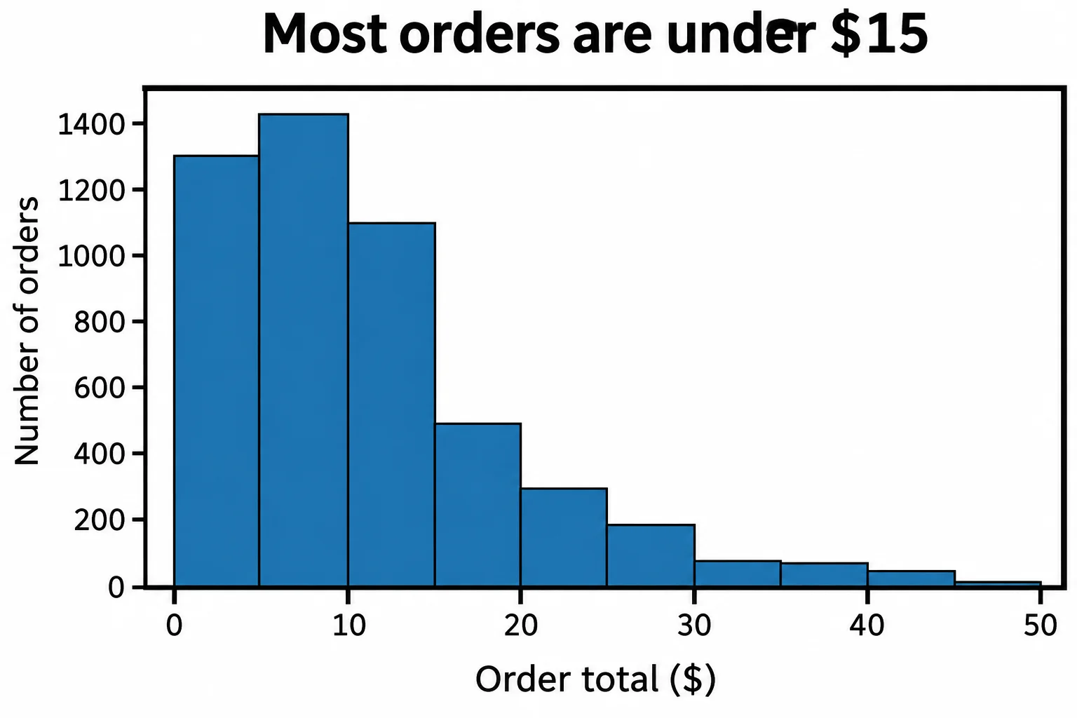
How many bins is right? Fewer, wider bins smooth the shape and can hide it; at bins=2, every chart looks like two blocks. More, narrower bins show detail, and with too many, each bar holds a handful of orders and the chart turns jagged. Try a few numbers, and keep the one that shows the shape most plainly.
The shape, in plain words
A histogram is read for its shape, and the shape is worth a sentence in plain words. Here: most orders are small, a single cone or two, under $15 (3,832 of the 5,000); then the bars fall away in a long tail to the right, a few family orders reaching $45 to $50.
That tail is what pulls the mean up. Every $48 order lifts the average, while the median, the middle order, stays at $8.75. In a statistics class this shape is called right-skewed. For a column like this, the median is the better "typical order", and the owner's family deal should be priced against the tail, not the average.
A histogram or a bar chart?
The bars look alike, and the two answer different questions:
- A bar chart has one bar for each category, such as a flavor. The bars have gaps between them, and their order is your choice (largest first, usually).
- A histogram has one bar for each range of a number. The bars touch, because each range ends where the next begins, and their order is fixed: the numbers run from small to large.
So scoops_sold by flavor is a bar chart, and order_total is a histogram. A column of whole numbers with only a few values, such as items (1 to 8), sits in between: orders["items"].value_counts().sort_index() counts each value, and a bar for each count reads well.
Check yourself
2 questions to try on the lesson page.
So what
When the question is "how are these values spread?", draw a histogram with bins you can say aloud, then describe its shape in words: where most values sit, and how far the tail reaches.