Several Charts on One Page: subplots and savefig
plt.subplots(2, 2, figsize=(10, 8), layout="constrained") makes one page with a grid of four Axes, each chart is drawn on its own Axes such as axs[0, 0], fig.suptitle gives the page a title, and fig.savefig saves it with dpi and bbox_inches="tight", as a PNG for a report or an SVG that stays sharp at any size.
Journeyman · Python · Updated
After this lesson you can
- Lay out several charts on one page with plt.subplots(2, 2), layout='constrained' and fig.suptitle
- Save a page of charts with fig.savefig, choosing dpi, bbox_inches='tight' and PNG or SVG
Key takeaways
- plt.subplots(2, 2) makes one Figure with a 2 by 2 grid of Axes, and axs[0, 0] is the top-left chart, axs[1, 1] the bottom-right one.
- figsize=(10, 8) sets the page's size in inches, and layout="constrained" keeps the charts' titles and labels from overlapping.
- fig.suptitle gives the whole page a title, above each chart's own.
- fig.savefig with dpi=150 and bbox_inches="tight" saves a sharp page with no wasted border. A PNG goes in reports and slides, an SVG stays sharp at any size.
One chart answers one question. A report usually has several questions, and the people reading it want the answers together, on one page: a one-page summary for a meeting, a figure in a lab report with four panels, a slide that compares a few things at once. Four separate image files get shuffled, resized and separated from each other. This lesson puts the charts on one page, and saves it.
The example is Clearwater City's recycling log, pickups.csv: one row for each of six neighborhoods in each month of 2024 and 2025, with tons_recycled, tons_trash and households among its columns. Curbside recycling pickup began in January 2025.
A page with a grid of charts
In matplotlib, the page is the Figure and each chart is an Axes. plt.subplots() with no numbers makes one of each; give it a number of rows and columns and it makes a grid:
import matplotlib.pyplot as plt
import pandas as pd

pickups = pd.read_csv("pickups.csv", parse_dates=["month"])
monthly = pickups.groupby("month")[["tons_recycled", "tons_trash"]].sum()
year_2025 = pickups[pickups["month"].dt.year == 2025]
by_neighborhood = year_2025.groupby("neighborhood")["tons_recycled"].sum().sort_values()

fig, axs = plt.subplots(2, 2, figsize=(10, 8), layout="constrained")
print(axs.shape)
(2, 2)
axs is a grid of Axes, 2 rows by 2 columns, and you pick one by its row and column, counting from 0: axs[0, 0] is top left, axs[0, 1] top right, axs[1, 0] bottom left, axs[1, 1] bottom right. figsize=(10, 8) makes the page 10 inches wide and 8 tall; the default, 6.4 by 4.8, is meant for one chart, and four on it would be cramped. layout="constrained" makes matplotlib fit each chart's title and labels into the space they need. Without it, one chart's x-axis labels can run into the title of the chart below.
A chart on each Axes, and a title for the page
Each chart is drawn the way you already know, on its own Axes:
top_left = axs[0, 0]
top_left.plot(monthly.index, monthly["tons_recycled"], marker="o")
top_left.set_title("Recycling rose after curbside pickup began")
top_left.set_ylabel("Recycled (tons)")
top_left.tick_params(axis="x", labelrotation=45)

top_right = axs[0, 1]
top_right.barh(by_neighborhood.index, by_neighborhood.values)
top_right.set_title("Downtown recycled the most in 2025")
top_right.set_xlabel("Recycled (tons)")

bottom_left = axs[1, 0]
bottom_left.scatter(pickups["households"], pickups["tons_recycled"], alpha=0.5)
bottom_left.set_title("Bigger neighborhoods recycle more")
bottom_left.set_xlabel("Households")
bottom_left.set_ylabel("Recycled (tons)")

bottom_right = axs[1, 1]
bottom_right.hist(pickups["tons_recycled"], bins=range(20, 70, 5))
bottom_right.set_title("Most months: 30 to 45 tons a neighborhood")
bottom_right.set_xlabel("Recycled in a month (tons)")
bottom_right.set_ylabel("Months")

fig.suptitle("Clearwater City recycling, 2024 to 2025")
plt.show()
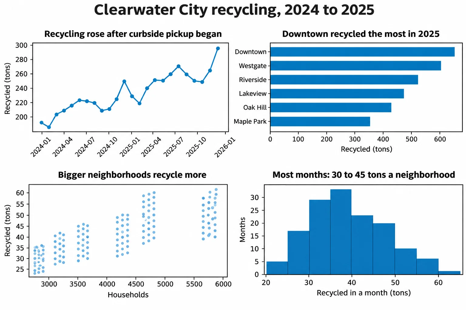
A short name for each Axes, such as top_left, makes the code easier to read than axs[0, 0] four times over. bins=range(20, 70, 5) gives the histogram a range every 5 tons, from 20 to 65. tick_params(axis="x", labelrotation=45) tilts one chart's date labels; fig.autofmt_xdate() would tilt every chart's, and only the top-left one has dates. fig.suptitle (read "sup title", short for super title) puts one title over the whole page, above each chart's own. Every chart still states its own finding; the page title says what they're all about.
Saving the page: savefig
fig.savefig saves the whole Figure, all four charts and both kinds of title, as one file:
fig.savefig("recycling-summary.png", dpi=150, bbox_inches="tight")
height, width, colors = plt.imread("recycling-summary.png").shape
print("Saved recycling-summary.png:", width, "by", height, "pixels")
Saved recycling-summary.png: 1517 by 1217 pixels
dpi=150 (dots per inch) sets how many pixels each inch of the page becomes: 10 inches at 150 dpi is about 1500 pixels across, sharp on a slide or a printed page. The default, 100, is fine on a screen. bbox_inches="tight" trims the empty border around the charts. plt.imread reads the saved picture back, and .shape gives its height, width and color channels, which is how you can check a file without opening it.
PNG or SVG
The ending of the file's name picks its type:
- PNG is a grid of pixels. It goes into a Word document, a slide, an email or a web page, and every program opens it. Its
dpidecides how sharp it is. - SVG stores the shapes and text themselves, not pixels, so it stays sharp at any size, and a web page can scale it to fit. It has no
dpito choose:
fig.savefig("recycling-summary.svg", bbox_inches="tight")
print("Saved recycling-summary.svg")
Saved recycling-summary.svg
For a report someone will open in an office program, save a PNG at 150 dpi. For a web page or a poster that will be printed large, an SVG keeps every line crisp.
Check yourself
2 questions to try on the lesson page.
So what
A page of charts with one title, saved as a single sharp file, keeps a set of answers together the way the reader needs them, in a meeting, a report or a slide.