Measuring Results Group by Group
One score for everyone hides how a model treats each group, so you split the test rows by group, count each group's own confusion matrix, and compare three rates, the selection rate, the true positive rate and the false positive rate, whose gaps are what Fairlearn's demographic parity and equalized odds ask to be zero.
Freelancer · AI Basics · Python · Updated
After this lesson you can
- Compute each group's selection rate, true positive rate and false positive rate from its own confusion matrix, by hand and in Python
- Compare groups by the gap in each rate, and tell demographic parity from equalized odds as Fairlearn's documentation defines them
Key takeaways
- The selection rate is the share of a group the model picks, (TP + FP) divided by the group's size.
- The true positive rate is the share of the group's qualified people it picks, TP / (TP + FN). The false positive rate is the share of the unqualified it picks, FP / (FP + TN).
- Demographic parity, as Fairlearn defines it, asks for equal selection rates. Equalized odds asks for equal true positive rates and equal false positive rates.
- A gap is the highest group's rate minus the lowest. It says how the model treats each group, not why, and it can move a lot with another test set, so measure it on more than one split.
The Summit Scholarship Fund's board read Where Bias Comes From and asks a plain question: does the screen treat North and South applicants the same? "Most of its invitations are right" doesn't answer it. Any time a model's guesses reach people, someone will ask how it does for each group of them, and the answer is a few rates per group, set side by side.
The example is still the fund's applicants.csv, from Exercise: Fairness Audit. Each code block is one notebook cell, run in order.
One score for everyone
This first cell trains the same screen as Where Bias Comes From: it learns from the old reviewers' invitations, with district left out. Then it checks the screen's 500 test invitations against qualified, the fund's own standard:
import pandas as pd
from sklearn.linear_model import LogisticRegression
from sklearn.model_selection import train_test_split
from sklearn.pipeline import make_pipeline
from sklearn.preprocessing import StandardScaler

applicants = pd.read_csv("applicants.csv")
features = ["gpa", "essay_score", "activities", "recommendation", "work_hours_per_week"]
train, test = train_test_split(applicants, test_size=0.25, random_state=42)
screen = make_pipeline(StandardScaler(), LogisticRegression())
screen.fit(train[features], train["invited_past"])
test = test.assign(invited=screen.predict(test[features]))
print("Test applicants:", len(test))
print("Invitations that match qualified:", round((test["invited"] == test["qualified"]).mean(), 3))
Test applicants: 500
Invitations that match qualified: 0.866
The answer to compare with is qualified, not invited_past. Scored against the old invitations, a screen that copied the old reviewers' habits perfectly would look perfect. Real data rarely has a column like qualified; when it doesn't, say plainly what your "actual" column is, because every rate below depends on it.
The 86.6% mixes both districts into one number. A screen can be right for most applicants and still wrong much more often for one group.
Three rates for each group
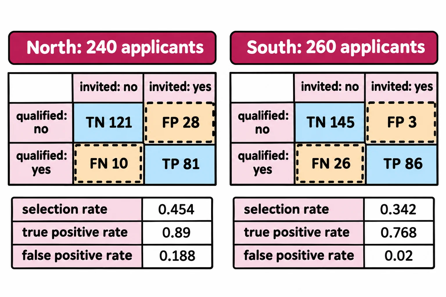
So split the test applicants by district, and give each district its own confusion matrix (The Confusion Matrix teaches the four counts). Qualified is the positive class: a true positive is a qualified applicant invited, a false negative a qualified one turned away.
from sklearn.metrics import confusion_matrix

rates = {}
for district, group in test.groupby("district"):
    tn, fp, fn, tp = confusion_matrix(group["qualified"], group["invited"], labels=[0, 1]).ravel().tolist()
    print(district, "applicants:", len(group), "TN:", tn, "FP:", fp, "FN:", fn, "TP:", tp)
    rates[district] = {
        "selection rate": (tp + fp) / len(group),
        "true positive rate": tp / (tp + fn),
        "false positive rate": fp / (fp + tn),
    }
North applicants: 240 TN: 121 FP: 28 FN: 10 TP: 81
South applicants: 260 TN: 145 FP: 3 FN: 26 TP: 86
labels=[0, 1] keeps every grid two by two, even for a group with no qualified applicants at all. Three rates come from each grid:
- The selection rate, (TP + FP) ÷ the group's size: the share of the group the screen invites.
- The true positive rate, TP ÷ (TP + FN), read "true positives over true positives plus false negatives": of the group's qualified applicants, the share invited. It's the recall from Precision and Recall, worked out inside one group.
- The false positive rate, FP ÷ (FP + TN): of the group's applicants who don't meet the standard, the share invited anyway.
for district, measures in rates.items():
    for measure, value in measures.items():
        print(district, measure, round(value, 3))
North selection rate 0.454
North true positive rate 0.89
North false positive rate 0.188
South selection rate 0.342
South true positive rate 0.768
South false positive rate 0.02
Now the rates say something a person can weigh. A qualified North applicant is invited 89% of the time, a qualified South applicant 76.8%. And 18.8% of North applicants who don't meet the standard are invited anyway, against 2% in South.
Two definitions of fair
Fairlearn, the Python library for this work, defines two goals with these rates. Demographic parity asks for equal selection rates across groups: whether you're invited shouldn't depend on your group. Equalized odds asks for two things at once: equal true positive rates and equal false positive rates. Among applicants who meet the standard, and again among those who don't, your group shouldn't change your chances. Each goal is measured by its gap, the highest group's rate minus the lowest:
for measure in ["selection rate", "true positive rate", "false positive rate"]:
    values = [measures[measure] for measures in rates.values()]
    print(f"{measure} gap: {max(values) - min(values):.3f}")
selection rate gap: 0.112
true positive rate gap: 0.122
false positive rate gap: 0.168
The selection rate gap, 0.112, is what Fairlearn calls the demographic parity difference. Its equalized odds difference is the larger of the other two gaps, here 0.168. A difference of 0 means the goal is met exactly.
Reading a gap honestly
A gap says how the screen treats each group, not why, and not what anyone meant. "The screen invites qualified South applicants less often" is the claim these numbers support: 76.8% against 89%.
Each rate also comes from a few hundred applicants, so a different test set can move it. This cell repeats the whole split, fit and count with seed 42 and four others:
for seed in [0, 1, 7, 42, 99]:
    tr, te = train_test_split(applicants, test_size=0.25, random_state=seed)
    model = make_pipeline(StandardScaler(), LogisticRegression()).fit(tr[features], tr["invited_past"])
    shares = te.assign(invited=model.predict(te[features])).groupby("district")["invited"].mean()
    print("random_state", seed, "selection rate gap:", round(shares["North"] - shares["South"], 3))
random_state 0 selection rate gap: 0.241
random_state 1 selection rate gap: 0.211
random_state 7 selection rate gap: 0.266
random_state 42 selection rate gap: 0.112
random_state 99 selection rate gap: 0.32
Every split invites North more often, but the size of the gap swings from 0.112 to 0.32, and the split this lesson used happens to show the smallest. One test set's gap is a rough measure. A gap that points the same way on every split is worth acting on; report its range, not only the friendliest number.
Do it: work out one district's three rates
The fund's board has ten South applicants from a pilot screen, and they want that district's three rates.
The inputs:
qualified: one number per applicant,1if they meet the fund's standard and0if not.invited: one number per applicant, in the same order,1if the screen invited them and0if not.
For example:
qualified = [1, 1, 1, 1, 0, 0, 0, 0, 0, 0]
invited = [1, 1, 1, 0, 1, 0, 0, 0, 0, 0]
| Count | Applicants | Total |
|---|---|---|
| TP: qualified and invited | 1st, 2nd, 3rd | 3 |
| FN: qualified, not invited | 4th | 1 |
| FP: not qualified, invited | 5th | 1 |
| TN: not qualified, not invited | 6th to 10th | 5 |
So the selection rate is (3 + 1) ÷ 10 = 0.4, the true positive rate is 3 ÷ (3 + 1) = 0.75, and the false positive rate is 1 ÷ (1 + 5) = 0.1666…, rounded to 0.167.
Your job: write district_rates(qualified, invited).
- It returns a dictionary with three keys:
"selection rate","true positive rate"and"false positive rate". - Each value is rounded to 3 decimal places with
round(value, 3). - The lists always hold at least one qualified applicant and at least one who isn't, so no rate divides by 0.
Practiced live on the lesson page: write the Python right there and check it.
Check yourself
2 questions to try on the lesson page.
So what
Fairness you can talk about starts with numbers you can check: each group's own counts, three rates from them, and the gaps that demographic parity and equalized odds ask to close.
Sources
- Fairlearn, Common fairness metrics, User Guide: demographic parity is achieved when the probability of a prediction doesn't depend on sensitive group membership, which for binary classification means equal selection rates across groups; equalized odds asks that groups have the same true positive rates and false positive rates; the demographic parity difference is the absolute difference between the highest and lowest selection rates; the equalized odds difference is the larger of the true positive rate difference and the false positive rate difference.
- Fairlearn, selection_rate, API reference: the fraction of predicted labels matching the "good" outcome.
- scikit-learn 1.9.1, confusion_matrix, API reference: entry i, j is the number of samples with true label i predicted as label j;
labelsselects or orders the labels that index the matrix; in binary classification, true negatives, false positives, false negatives and true positives come out in that order from.ravel(). - scikit-learn, Metrics and scoring, User Guide: recall is tp / (tp + fn); the true positive rate is the fraction of true positives out of the positives, and the false positive rate the fraction of false positives out of the negatives.