How a Guess Changes with One Feature
Changing one feature of a home while keeping the rest the same, and watching the model's guess, gives that home's individual line, and averaging every home's line gives the partial dependence, which PartialDependenceDisplay.from_estimator draws with kind='both', but it shows how the model behaves, not cause and effect, and it can't be trusted where the data is thin.
Freelancer · AI Basics · Python · Updated
After this lesson you can
- Compute and draw partial dependence and individual lines with PartialDependenceDisplay.from_estimator and kind='both', and read what they show
- Explain why partial dependence shows the model's behavior, not cause and effect, and why it can't be trusted where the data is thin
Key takeaways
- An individual line (ICE) changes one feature of one home, keeps everything else as it was, and plots the model's guess at each value.
- Partial dependence is the average of every home's individual line, the model's average guess as one feature changes.
- PartialDependenceDisplay.from_estimator draws them, and kind='both' shows the individual lines with the average on top.
- It shows how the model behaves, not cause and effect, and it assumes the feature can change while the others stay put.
- Where the training data is thin, the line rests on few examples, and past the largest example a tree model can only stay flat.
A Greenway customer planning an addition asks: if my house were bigger, how much more would the estimate be? Permutation importance (Permutation Importance) said the forest leans on size more than anything else, but not how: does the guess climb steadily, level off, or jump? You'll need that answer whenever someone asks "what if this were different?" about a model's guess.
The example is Greenway's home_energy.csv, from Exercise: Explain the Energy Bill. Each code block is one notebook cell, run in order: the first one loads the data and trains the forest from Permutation Importance.
One home, many sizes
Take one test home and ask the model about copies of it that differ only in size:
import pandas as pd
from sklearn.compose import make_column_transformer
from sklearn.ensemble import RandomForestRegressor
from sklearn.model_selection import train_test_split
from sklearn.pipeline import make_pipeline
from sklearn.preprocessing import OneHotEncoder

homes = pd.read_csv("home_energy.csv")
features = ["size_sqft", "year_built", "insulation", "heating", "occupants", "has_pool"]
X_train, X_test, y_train, y_test = train_test_split(
    homes[features], homes["monthly_bill"], test_size=0.2, random_state=42)
prep = make_column_transformer(
    (OneHotEncoder(handle_unknown="ignore"), ["insulation", "heating"]),
    remainder="passthrough",
    verbose_feature_names_out=False,
)
forest = make_pipeline(prep, RandomForestRegressor(n_estimators=200, random_state=0))
forest.fit(X_train, y_train)

home = X_test.iloc[[0]]
print(home.to_string(index=False))
 size_sqft  year_built insulation heating  occupants  has_pool
      1770        1954       fair     gas          4         0
copies = pd.concat([home] * 5, ignore_index=True)
copies["size_sqft"] = [1000, 2000, 3000, 4000, 5000]
for size, guess in zip(copies["size_sqft"], forest.predict(copies)):
    print(size, "square feet:", round(guess, 2))
1000 square feet: 141.21
2000 square feet: 189.66
3000 square feet: 216.73
4000 square feet: 222.54
5000 square feet: 222.54
The guess climbs from 1,000 to 3,000 square feet, then stops: 4,000 and 5,000 get the same $222.54. Those five points, joined up, are this home's individual line. Your textbook may call it an individual conditional expectation line, ICE for short.
Every home, then the average
Do that for every home and average the lines at each size, and you get the model's average guess as size changes, with every other feature as it was: the partial dependence. scikit-learn's partial_dependence computes it, but the first try stops:
from sklearn.inspection import partial_dependence

result = partial_dependence(forest, X_train, ["size_sqft"])
ValueError: The column 'size_sqft' contains integer data. Partial dependence plots are not supported for integer data: this can lead to implicit rounding with NumPy arrays or even errors with newer pandas versions. Please convert numerical features to floating point dtypes ahead of time to avoid problems.
The sizes are whole numbers, and scikit-learn wants the number columns as floats (numbers with a decimal point) before it fills in the sizes to try. astype converts them:
X_float = X_train.astype({"size_sqft": float, "year_built": float, "occupants": float})
result = partial_dependence(forest, X_float, ["size_sqft"], grid_resolution=5)
for size, average in zip(result["grid_values"][0], result["average"][0]):
    print(size, "square feet:", round(average, 2))
1010.0 square feet: 138.69
1437.5 square feet: 157.42
1865.0 square feet: 176.28
2292.5 square feet: 193.96
2720.0 square feet: 219.61
grid_resolution=5 asks for five evenly spaced sizes (the default is 100). They run from 1,010 to 2,720 square feet, not from the smallest home to the largest: by default the range is cut at the 5th and 95th percentiles of the column, so the few homes at each end don't stretch it. (A column with fewer different values than the grid asks for, like the year built's 75 years against the default 100, is tried at every value it has instead.) Across that range, the model's average guess rises about $81.
Drawing it
PartialDependenceDisplay.from_estimator computes the lines and draws them with matplotlib:
import matplotlib.pyplot as plt
from sklearn.inspection import PartialDependenceDisplay

PartialDependenceDisplay.from_estimator(
    forest, X_float, ["size_sqft", "year_built"],
    kind="both", subsample=50, random_state=0,
)
plt.show()
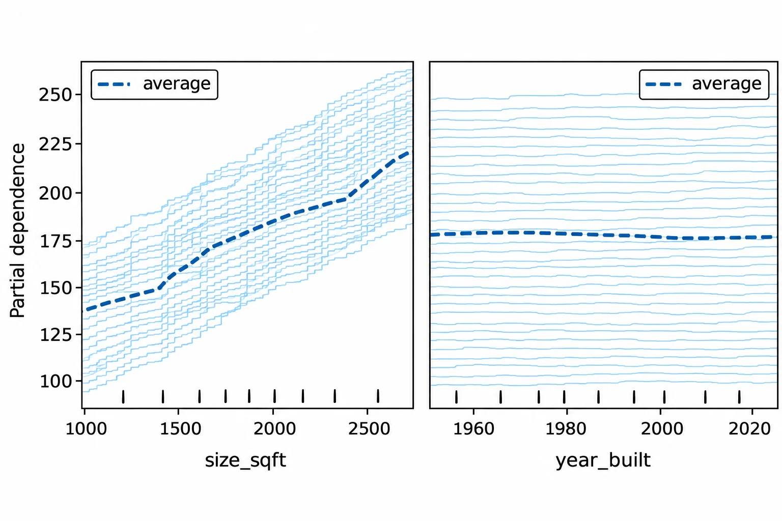
kind="both" draws each home's individual line, thin, with the average on top, dashed; kind="average", the default, draws only the average. subsample=50 draws 50 homes' lines, chosen with random_state=0, so the chart stays readable; the average still uses every home. The short ticks along the bottom are the deciles: each tenth of the training homes falls between two ticks.
Read the left chart: the average climbs, and the individual lines mostly climb together, roughly parallel. Lines that crossed or bent differently would mean the model treats different homes' size differently. Read the right one: the year built barely moves the guess at all, which matches its permutation importance of about zero.
What it shows, and what it doesn't
It shows the model, not the world. "The average guess rises $81 from 1,010 to 2,720 square feet" is a fact about this forest. It doesn't promise that an addition raises a real bill by that much. In this made-up data the seed script planted $0.045 a square foot, and the forest came close; real data has no answer key.
It assumes one feature can change while the rest stay put. Each line keeps the year built and the insulation as they were. When features move together, that makes homes that hardly exist: scikit-learn's guide warns that with correlated features the lines are computed on absurd data points.
It can't be trusted where the data is thin:
print("Training homes over 3,000 square feet:", (X_train["size_sqft"] > 3000).sum())
print("Largest training home:", X_train["size_sqft"].max())
Training homes over 3,000 square feet: 8
Largest training home: 3400
Only 8 of 560 training homes are over 3,000 square feet, so that end of the line rests on 8 bills. Past 3,400, the forest has seen nothing at all: a tree can only guess an average of bills it learned from, so the guess stays flat, which is why 4,000 and 5,000 square feet got the same $222.54. The seed script's rule would add about $72 between 3,400 and 5,000 square feet. Guessing past the data you learned from is called extrapolation, and a tree model can't do it (Regression Trees).
Check yourself
2 questions to try on the lesson page.
So what
Partial dependence and individual lines answer "what if this were different?" about a model: how its guess moves as one feature changes, on average and home by home, as long as you say it's the model talking and keep to where the data is.
Sources
- scikit-learn, Partial Dependence and Individual Conditional Expectation plots, User Guide. Partial dependence plots: the dependence between the target response and a feature, marginalizing over the values of all the other features, the expected response as a function of the feature. Individual conditional expectation (ICE) plot: one line per sample, showing how that sample's prediction changes as the feature changes; a partial dependence line can hide differences an ICE plot shows, so the two are recommended together, with
kind='both'. Both assume the feature is independent of the others; with correlated features, they are computed on absurd data points. - scikit-learn 1.9.1, PartialDependenceDisplay, API reference:
from_estimatordraws one-way partial dependence;kindis'average'(the default),'individual'or'both';subsample(default 1000) limits the ICE lines drawn, while the full dataset is still used for the average, andrandom_statecontrols which samples are chosen;grid_resolution(default 100) andpercentiles(default (0.05, 0.95)) set the grid; the deciles of the feature's values are shown on the x-axis. - scikit-learn 1.9.1, partial_dependence, API reference: returns
grid_values, the values tried (as many asgrid_resolutionor the column's number of unique values, whichever is smaller), andaverage, the predictions averaged over the samples at each value (andindividualfor ICE). - scikit-learn, Decision Trees, User Guide: with the default squared-error criterion, a leaf predicts the mean of its training targets; tree predictions are piecewise constant approximations, neither smooth nor continuous, so trees are not good at extrapolation.