How Two Columns Move Together
A scatter plot shows whether two columns move together, and Pearson's correlation, read "r", puts it in one number from -1 to 1 (statistics.correlation for two lists, df.corr() for a whole table), but r only measures straight-line patterns, a weak r can hide a real effect, and moving together isn't causing.
Apprentice · AI Basics · Python · Updated
After this lesson you can
- Measure how two columns move together with statistics.correlation or df.corr(), and read r from -1 to 1 as strength and direction
- Explain what a correlation can't show, a curved pattern, a cause, or an effect that other columns hide
Key takeaways
- A scatter plot puts one dot per row, one column across and one up, so you can see whether the two move together.
- Pearson's correlation r runs from -1 to 1. Near 1, both rise together; near -1, one falls as the other rises; near 0, no straight-line pattern.
- statistics.correlation works out r for two lists, and df.corr() works it out for every pair of number columns in a table.
- r only measures straight-line patterns, so a perfect curve can score 0, and one column's r can't see the other columns.
- Correlation is not causation. Bedrooms go with higher rent because they go with bigger apartments, not because a bedroom adds rent.
Riverside's listings have six columns that could help guess the rent. Which ones are worth a model's attention? You can't tell from reading 300 rows, and guessing from what "should" matter is how people end up surprised. Measuring how each column moves with the label is the first look at a new dataset, before any model, and you'll do it every time you choose features.
The example is Riverside Apartments' listings.csv, from Exercise: Know Your Listings. The code blocks are notebook cells, run in order.
See it first: a scatter plot
A scatter plot draws one dot per row: one column across the bottom, the other up the side. Here are size against rent, and floor against rent:
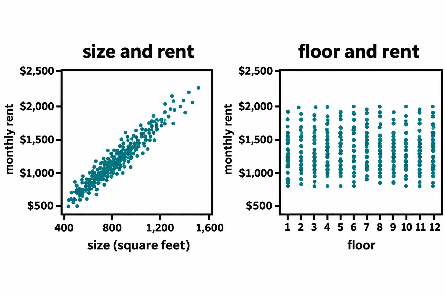
On the left, bigger apartments rent for more, with the dots in a tight band. On the right, every floor has cheap and expensive apartments: no pattern at all.
One number for it: the correlation r
Correlation turns that picture into one number. The usual kind, Pearson's correlation, read "r", runs from −1 to 1. Here is the idea behind it. For each apartment, ask how far its size is above or below the average size, in standard deviations (from The Middle and the Spread), and the same for its rent. Multiply the two. When a big apartment has a high rent, both are above average and the product is positive; a small, cheap one gives two negatives, also positive. Average the products (dividing by one less than the count, as the standard deviation does), and that's r:
- near 1: the dots lie close to a line rising to the right;
- near −1: close to a line falling to the right, one column going down as the other goes up;
- near 0: no straight-line pattern.
Python's statistics.correlation does the arithmetic:
import csv
import statistics

with open("listings.csv", newline="") as file:
    listings = list(csv.DictReader(file))

sizes = [int(listing["size_sqft"]) for listing in listings]
bedrooms = [int(listing["bedrooms"]) for listing in listings]
floors = [int(listing["floor"]) for listing in listings]
rents = [int(listing["monthly_rent"]) for listing in listings]
print("Size and rent:", round(statistics.correlation(sizes, rents), 3))
print("Floor and rent:", round(statistics.correlation(floors, rents), 3))
Size and rent: 0.905
Floor and rent: -0.004
Size and rent: strong. Floor and rent: as close to nothing as real numbers get. "Strong" and "weak" are rough words, not rules; read r beside the scatter plot.
Every column at once: df.corr()
pandas works out r for every pair of number columns with corr(). The ID is text, and corr() stops with a ValueError on a text column, so the code drops it first, and ["monthly_rent"] picks out each column's r with the rent:
import pandas as pd

table = pd.read_csv("listings.csv")
table.drop(columns="listing_id").corr()["monthly_rent"].round(2)
size_sqft              0.91
bedrooms               0.71
bathrooms              0.63
minutes_to_downtown   -0.23
has_parking            0.06
floor                 -0.00
monthly_rent           1.00
Name: monthly_rent, dtype: float64
Rent's r with itself is 1, as any column's is. minutes_to_downtown is negative: the farther out, the lower the rent.
What r can't tell you
Only straight lines. These five points lie on a perfect U-shaped curve, and r says nothing's there:
xs = [1, 2, 3, 4, 5]
ys = [4, 1, 0, 1, 4]
print("r:", statistics.correlation(xs, ys))
r: 0.0
An r near 0 means no straight-line pattern, so look at the scatter plot before you call two columns unrelated.
Not a cause. Bedrooms have r = 0.71 with rent, yet the seed script that made this data adds nothing to the rent for a bedroom. Bedrooms follow size:
print("Size and bedrooms:", round(statistics.correlation(sizes, bedrooms), 2))
Size and bedrooms: 0.78
Bigger apartments have more bedrooms and higher rents, so bedrooms and rent move together without one causing the other. Correlation is not causation: an owner who puts up a wall to make a second bedroom hasn't added a square foot.
One column at a time. has_parking has r = 0.06, close to none, but the seed script adds $120 a month for a parking space. Sizes swing over a thousand square feet and drown out that smaller effect, which r, looking at one column at a time, can't separate. A weak r doesn't prove a feature useless. Module 2's models look at the features together.
Do it: work out r by hand
Before trusting statistics.correlation, you'd like to see the arithmetic work on a few Riverside listings.
The inputs:
xs: one column's values, such as sizes.ys: another column's values for the same rows, in the same order, such as rents. Both lists have the same length, at least two values each, and neither has all its values the same.
For example, xs = [600, 700, 800, 900, 1000] and ys = [1100, 1000, 1300, 1200, 1400]. The means are 800 and 1,200, and both standard deviations are 158.11 (statistics.stdev):
| Size | Standard deviations from 800 | Rent | Standard deviations from 1,200 | Product |
|---|---|---|---|---|
| 600 | −1.265 | 1,100 | −0.632 | 0.8 |
| 700 | −0.632 | 1,000 | −1.265 | 0.8 |
| 800 | 0 | 1,300 | 0.632 | 0 |
| 900 | 0.632 | 1,200 | 0 | 0 |
| 1,000 | 1.265 | 1,400 | 1.265 | 1.6 |
The products add up to 3.2, and 3.2 ÷ (5 − 1) = 0.8. So correlation(xs, ys) returns 0.8.
Your job: write correlation(xs, ys) the way the table does it.
- For each pair, work out how many standard deviations
xis from the mean ofxs: (x − mean) ÷ standard deviation. Do the same forywithys. - Multiply the two, add up the products, and divide by the count minus one.
- Return the result rounded to 3 decimal places.
- You may use
statistics.fmeanandstatistics.stdevfor the means and standard deviations.
Practiced live on the lesson page: write the Python right there and check it.
Check yourself
2 questions to try on the lesson page.
So what
Correlation is a quick, honest first look at which columns go with the label, as long as you remember what it can't see: curves, causes, and effects that other columns hide.
Sources
- Python documentation, statistics.correlation: Pearson's correlation coefficient r, between −1 and +1, measures the strength and direction of a linear relationship; both inputs must be the same length, at least two values, and not constant;
method='ranked'gives Spearman's rank correlation instead. - pandas 3.1.1, DataFrame.corr, API reference: pairwise correlation of columns, Pearson's by default, excluding missing values;
numeric_onlyisFalseby default, so every column must hold numbers: a text column such as an ID has to be dropped first. - scikit-learn, Glossary of Common Terms and API Elements, feature: a column of the data matrix; scikit-learn's estimators assume features are numeric.