Your First pandas Table
pandas reads a whole CSV file into a DataFrame, a table you can ask questions, and a few lines then show what's in it, pick out a column, keep the rows that match a condition and total a column for each group.
Apprentice · Python · Updated
After this lesson you can
- Load a CSV file into a pandas DataFrame with read_csv, and look at it with head, info and describe
- Pick a column of a DataFrame, keep the rows that match a condition, and total a column by group with groupby
Key takeaways
- pd.read_csv reads a whole CSV file into a DataFrame, a table with named columns and a label for each row, called its index.
- head() shows the first five rows, info() each column's type and how many values it holds, and describe() the count, mean, smallest and largest of each number column.
- One column, such as week["sales"], is a Series, and sum(), mean() and max() work on the whole column at once.
- A condition inside square brackets, such as week[week["store"] == "Harbor"], keeps only the rows where it's True.
- groupby("store")["sales"].sum() totals the sales for each store in one line, and idxmax() names the store with the biggest total.
Which store sold the most last month? Which homework did the class find hardest? What was the average of those 200 lab readings? Each is a question answered with numbers from a table, and answering them is what data analysis is. It's one of the most common jobs Python does after class, in offices, labs and small businesses alike, and this lesson gives you a first taste of the tool most Python analysts use: pandas.
The example is Bean Street Coffee, a small chain with three stores (Downtown, Campus and Harbor), and its sales for the first week of October: one row for each store on each day. The sales are our own made-up numbers.
One question, one loop
The week's sales are in a CSV file, sales.csv, with the cups sold and the sales in dollars:
date,store,cups,sales
2026-10-01,Downtown,265,1205
2026-10-01,Campus,275,1195
2026-10-01,Harbor,136,675
2026-10-02,Downtown,303,1420
2026-10-02,Campus,280,1233
2026-10-02,Harbor,179,883
2026-10-03,Downtown,208,974
2026-10-03,Campus,118,498
2026-10-03,Harbor,280,1325
2026-10-04,Downtown,166,761
2026-10-04,Campus,121,527
2026-10-04,Harbor,296,1426
2026-10-05,Downtown,294,1395
2026-10-05,Campus,255,1120
2026-10-05,Harbor,177,859
2026-10-06,Downtown,259,1209
2026-10-06,Campus,221,954
2026-10-06,Harbor,148,708
2026-10-07,Downtown,268,1263
2026-10-07,Campus,249,1035
2026-10-07,Harbor,175,842
Rosa, who owns the chain, asks which store sold the most this week. With the csv module from CSV Files: Tables in Plain Text, that's a dictionary and a loop:
import csv

totals = {}
with open("sales.csv", newline="", encoding="utf-8") as file:
    for row in csv.DictReader(file):
        store = row["store"]
        totals[store] = totals.get(store, 0) + int(row["sales"])
print(totals)
{'Downtown': 8227, 'Campus': 6562, 'Harbor': 6718}
It works. Then Rosa asks which day was the busiest, and how many cups Harbor sold. Each new question is another loop, another dictionary and another int() to remember. Analysts ask dozens of questions of the same table, so they use a tool that already knows how.
pandas: a table you can ask questions
pandas is a package for working with tables of data. It doesn't come with Python, so install it into a virtual environment, as Virtual Environments and pip shows. In a new folder holding sales.csv, with the environment active (matplotlib is for the next lesson's chart):
pip install pandas==3.1.1 matplotlib==3.11.2
Then read the file:
import pandas as pd

week = pd.read_csv("sales.csv")
print(week.head())
         date     store  cups  sales
0  2026-10-01  Downtown   265   1205
1  2026-10-01    Campus   275   1195
2  2026-10-01    Harbor   136    675
3  2026-10-02  Downtown   303   1420
4  2026-10-02    Campus   280   1233
import pandas as pd brings pandas in under the short name pd (read "p d"), which nearly everyone uses. pd.read_csv reads the whole file into a DataFrame: a table inside your program, like one sheet of a spreadsheet, with named columns. The numbers down the left are its index, a label for each row, counting from 0. head() shows the first five rows, the quick look you take before anything else. pandas also turned the cups and sales into numbers on its own, with no int().
To try an idea without a file, you can also build a small DataFrame in code, from a dictionary whose keys are the column names and whose values are lists, one value per row: pd.DataFrame({"store": ["Downtown", "Campus"], "sales": [1205, 1195]}).
What's in the table: info and describe
Two more methods tell you what you're working with before you trust it:
import pandas as pd

week = pd.read_csv("sales.csv")
week.info()
print(week.describe())
<class 'pandas.DataFrame'>
RangeIndex: 21 entries, 0 to 20
Data columns (total 4 columns):
 #   Column  Non-Null Count  Dtype
---  ------  --------------  -----
 0   date    21 non-null     str
 1   store   21 non-null     str
 2   cups    21 non-null     int64
 3   sales   21 non-null     int64
dtypes: int64(2), str(2)
memory usage: 804.0 bytes
             cups        sales
count   21.000000    21.000000
mean   222.523810  1024.142857
std     62.132615   287.677647
min    118.000000   498.000000
25%    175.000000   842.000000
50%    249.000000  1035.000000
75%    275.000000  1233.000000
max    303.000000  1426.000000
info() prints a list of the columns: how many values each one has (21 non-null means no blanks) and its type, int64 for whole numbers and str for text. (Older pandas, and many answers online, show text as object.) describe() sums up each number column: how many values, the mean (the average), the smallest and the largest. The 50% row is the middle value: half of the rows have sales of $1,035 or less. std, the standard deviation, says how spread out the values are: the bigger it is, the more the rows differ from the mean.
One column and a filter
A DataFrame's column, picked by its name in square brackets, is a Series: one column of values, keeping the table's index. Its methods work on the whole column at once:
import pandas as pd

week = pd.read_csv("sales.csv")
print(week["sales"].sum())
print(week["cups"].max())
harbor = week[week["store"] == "Harbor"]
print(harbor)
21507
303
          date   store  cups  sales
2   2026-10-01  Harbor   136    675
5   2026-10-02  Harbor   179    883
8   2026-10-03  Harbor   280   1325
11  2026-10-04  Harbor   296   1426
14  2026-10-05  Harbor   177    859
17  2026-10-06  Harbor   148    708
20  2026-10-07  Harbor   175    842
The harbor line is a filter. week["store"] == "Harbor" checks every row and gives True or False for each; put inside week[...], it keeps the rows where it's True. Read it as "the rows of week where store is equal to Harbor". The index still shows each row's place in the whole table.
Totals by group: groupby
Rosa's first question takes one line:
import pandas as pd

week = pd.read_csv("sales.csv")
totals = week.groupby("store")["sales"].sum()
print(totals)
print("Top store:", totals.idxmax())
store
Campus      6562
Downtown    8227
Harbor      6718
Name: sales, dtype: int64
Top store: Downtown
Picture sorting the week's receipts into three trays, one per store, then adding up each tray. groupby("store") makes the trays, ["sales"] picks the column to add, and .sum() totals each one. The result is a Series whose index is the store names, in A-to-Z order. idxmax() (read "index of the max") gives the label of the largest value: Downtown.
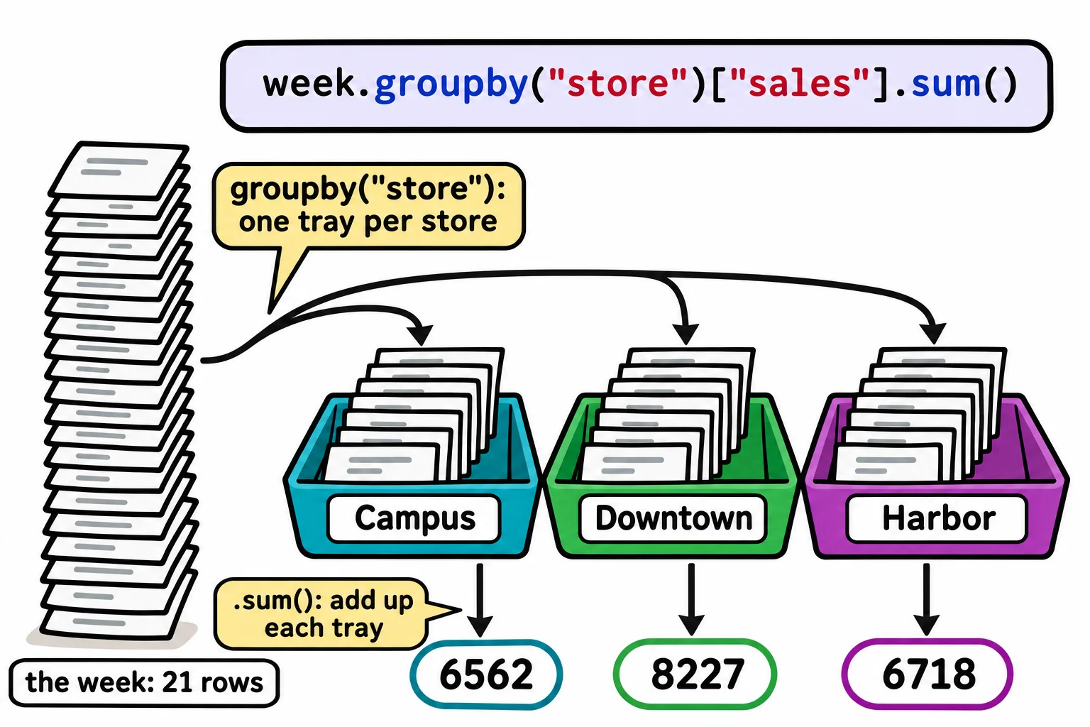
Analysts often run lines like these in a notebook, a file where each result shows right under the code that made it. This course works in .py files, which run the same code.
Check yourself
2 questions to try on the lesson page.
So what
A question about a table, such as which store sold the most, is one line of pandas instead of a loop, which is why analysts can ask so many of them.